Choosing a GPU for AI Workloads: The Full Placement Guide
Ask most teams how they chose their GPU and you'll hear a version of the same story: someone compared spec sheets, someone else checked hourly prices, and the team picked the card that looked right for "AI workloads" in general.
That instinct isn't wrong — spec comparisons matter, and the price gap between a T4 and an H100 is large enough that getting it wrong is expensive in either direction.
But "which GPU should we get" is only half the decision, and usually the smaller half. Every AI workload actually forces two choices:
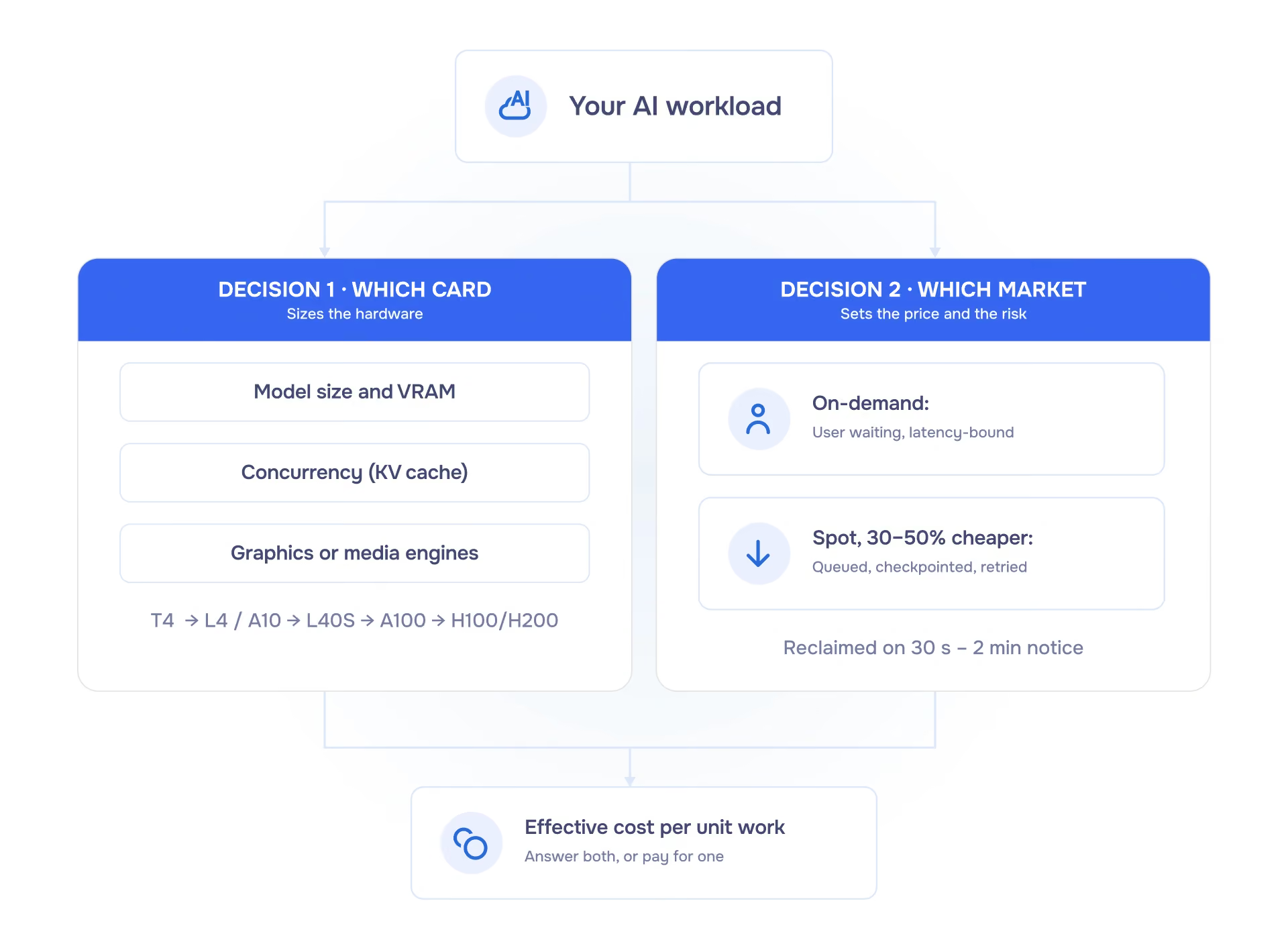
Which card — driven by model size, VRAM, concurrency, and whether the workload has a graphics or media component.
Which procurement model — on-demand capacity for anything user-facing and latency-sensitive, spot or preemptible capacity for anything that can be queued, checkpointed, and retried.
Teams that only make the first choice end up paying on-demand prices for batch jobs that would tolerate interruption, or discovering that the "best" card for their model has no available capacity in their region.
This guide walks you through how to make that decision properly across 12 common workload types — not just picking a GPU, but aligning the card, the workload shape, and the market you run it in.
Spec sheets rank GPUs by TFLOPs, but LLM inference doesn’t usually run out of compute. It typically runs out of memory capacity and bandwidth first. Four numbers do most of the deciding.
When thinking about GPU memory in LLM inference, it helps to separate two distinct components: the model weights and the KV cache. Both matter, but they behave very differently in practice.
The memory required for the model weights is relatively straightforward to estimate. It’s simply the number of parameters multiplied by the precision used to store them. At FP16, each parameter takes 2 bytes. That means an 8B parameter model requires roughly 16 GB of memory, while a 70B model needs around 140 GB. This is the baseline cost just to load the model into memory, before serving a single request. Techniques like INT4 quantization reduce this significantly, down to roughly 0.5 bytes per parameter, which is often what allows a model to fit on a smaller class of GPU.
The more subtle, and frequently underestimated, component is the KV cache. This is the attention state the model maintains for each active request, and it grows linearly with the length of the input (and generated output). Unlike weights, which are fixed, the KV cache scales dynamically with usage.
For a 7–8B class model at FP16, the KV cache is typically on the order of hundreds of KBs per token (roughly 100–300 KB, depending on architecture and implementation). This adds up quickly. A single 4k-token request can consume on the order of 1–2 GB of additional memory. With ten such requests running concurrently, that becomes 10–20 GB, often exceeding the memory footprint of the model itself.
This distinction leads to a common but critical misunderstanding: “the model fits” is not the same as “the workload fits.” A GPU that can hold the model weights may still run out of memory once real-world usage is factored in.
In practice, this is why increasing context length or concurrency can quickly push deployments into higher GPU tiers. It also explains the design of newer hardware like the H200, whose 141 GB of memory is not just about accommodating larger models, but about supporting realistic, high-concurrency workloads without running into memory limits.
While model size determines whether a workload fits in memory, memory bandwidth largely determines how fast it runs, especially during token generation.
During the decode phase (when the model generates tokens one by one), inference is primarily bandwidth-bound. Each new token requires repeatedly reading the model’s weights from GPU memory. Because of this, sustained token generation speed tends to scale with memory bandwidth: the faster the GPU can move data, the more tokens per second it can produce.
This is why GPUs with higher bandwidth deliver higher throughput in practice. For example, an L4 provides on the order of ~300 GB/s of memory bandwidth, an A10 around ~600 GB/s, an L40S ~864 GB/s, an A100 (80GB) roughly ~2 TB/s, and an H100 ~3.3 TB/s. While real-world performance depends on kernels and batching, the relationship between bandwidth and decode throughput is often close to linear.
The prefill phase—processing the initial prompt—is different. Here, the model can parallelize computation across all input tokens, making the workload more compute-bound than bandwidth-bound. As a result, improvements in raw compute (e.g., tensor cores, FLOPs) tend to have a greater impact on prompt processing speed than on token generation speed.
This split between prefill and decode has an important implication for performance evaluation. First-token latency (how quickly the model begins responding) is influenced more by compute performance, while inter-token latency (how quickly subsequent tokens are generated) depends more on memory bandwidth.
In practice, this means benchmarking a single request in isolation can be misleading. Real workloads involve concurrency, queueing, and varying context lengths. To understand actual performance, it’s important to measure both p50 and p95 latency for first-token and per-token generation under realistic load, rather than relying on idealized, single-request demos.
Continuous batching (vLLM, TGI) is how one card serves many users, but every concurrent request holds its own KV cache. And that memory usage scales linearly with the number of active requests.
Your real capacity per card is (VRAM − weights) ÷ KV-per-request. This determines how many requests you can serve concurrently on a single card. It is this number—not peak FLOPs or even raw bandwidth—that ultimately dictates whether a workload fits.
This is also where deployment decisions emerge. If the available memory cannot support the desired concurrency and context length, you are forced to either scale up to a larger GPU with more memory, or scale out across multiple GPUs and distribute requests.
Importantly, this calculation should be treated as a floor check, not a precise capacity plan. Modern serving frameworks use a range of optimizations—such as more efficient KV cache management, paging, and sharing—that can improve effective utilization beyond naive estimates.
But the inverse is more critical: if the workload does not fit even under this simplified calculation, no amount of serving-layer optimization will make it viable.
For GPU instances, spot capacity typically runs 30–50% below on-demand — less generous than the discounts people remember from CPU spot — and providers reclaim it on 30 seconds' to two minutes' notice depending on the cloud. Any stage that can be queued, checkpointed, and retried — embedding jobs, batch scoring, synthetic generation, tolerant training runs — belongs there.
Anything with a user waiting on the response doesn't. One caveat that surprises teams: for the highest-demand cards, spot barely exists. H100 spot availability is intermittent at best, because on-demand buyers absorb the capacity first, so a cost plan built on "H100s, but spot" is usually a plan built on capacity you won't get.
Training operates under a very different memory model than inference. In addition to the model weights, training requires storing gradients and optimizer state. With common setups like mixed-precision Adam, this brings total memory usage to roughly ~16 bytes per parameter, compared to ~2 bytes for FP16 inference.
This is why training workloads are typically confined to high-memory, high-bandwidth GPUs like the NVIDIA A100 and NVIDIA H100, even when the resulting model can be served comfortably on smaller hardware such as an L4.
T4 — 16 GB, ~320 GB/s.
Development, testing, lightweight or legacy inference. Cheap enough to validate a pipeline before you scale it; enough VRAM for quantized 7B-class models with modest context.
L4 — 24 GB, ~300 GB/s — and A10 — 24 GB, ~600 GB/s.
The production default for small-to-mid model inference (7B–13B, especially quantized), embeddings, and video work: the L4's NVENC/NVDEC engines make it a strong transcoding and video-analytics card. Note the bandwidth gap between the two — at equal VRAM, the A10 decodes meaningfully faster.
L40S — 48 GB, ~864 GB/s, strong graphics and media capability.
The general-purpose step up: 13B-class models at FP16 with real KV headroom, quantized 70B-class models, higher concurrency, and anything with a rendering or video component.
A100 — 40 or 80 GB (HBM2e, ~1.6–2 TB/s).
Large-model serving and demanding latency SLAs; still the workhorse for training, where the ~16-bytes-per-parameter budget lives.
H100 — 80 GB, ~3.3 TB/s — and H200 — 141 GB, ~4.8 TB/s.
The throughput ceiling and the VRAM ceiling respectively. The H200 isn't "a faster H100" so much as the answer when the constraint is memory itself: long context windows, large batches, very large models.
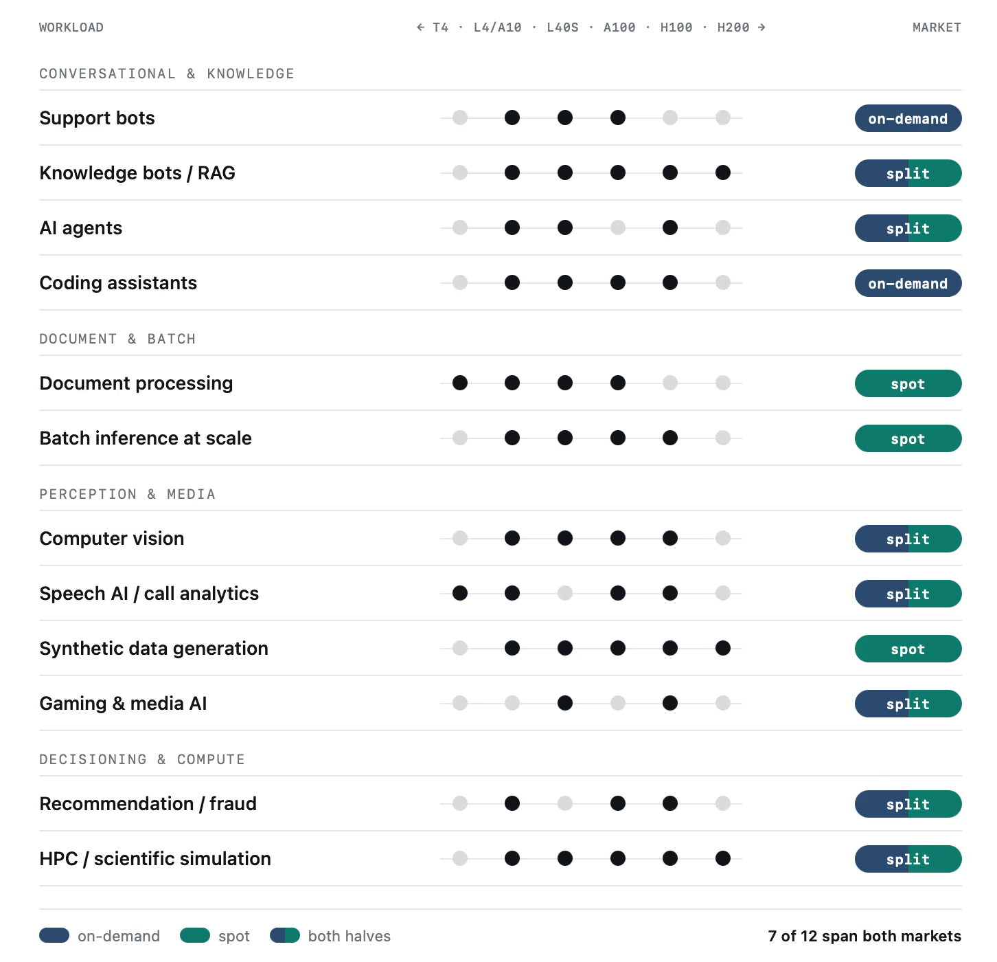
Support bots. A support bot is an inference system, not a training system: it accepts a question, retrieves context from your knowledge base, calls an LLM, and returns a grounded answer. For self-hosted quantized models at moderate traffic, an L4 or A10 is enough. Heavier models or high concurrency call for an L40S or A100.
Placement: on-demand. Users are waiting on the response.
Internal knowledge bots / RAG. RAG splits cleanly into two phases with different infrastructure profiles.
Placement: spot for ingestion and indexing, on-demand for serving. This is the cleanest example of one workload needing two procurement models.
AI agents. An agent is an orchestration: LLM plus tools, API calls, memory, sometimes code execution. The GPU sits at the inference endpoint, not under the whole workflow — and if the agent calls an external model API, there may be no GPU requirement at all.
Self-hosted agent inference usually lands on L4/L40S, with H100 reserved for heavy reasoning pipelines or high throughput. Worth calibrating ambition against the market here: McKinsey's 2025 State of AI survey found 62% of organizations at least experimenting with AI agents, but only 23% scaling them in any function. The gap between experimentation and production is most likely an infrastructure and governance gap, not a model gap.
Placement: on-demand for production agents, spot for async and background jobs.
AI coding assistants. Same inference pattern as support bots, different context: repository code, documentation, tickets. Self-hosting makes sense when data control matters or third-party API dependency doesn't.
Lightweight or quantized coding models run on L4/A10; larger models, bigger context windows, or many concurrent developers push toward L40S, A100, or H100.
Placement: on-demand. Developers notice latency.
Document processing. In practice this is a pipeline — PDF loading, OCR, layout parsing, classification, entity extraction, summarization — and the bottleneck is often I/O and the task queue, not the GPU.
L4, A10, or even T4 cover most OCR and classification stages. L40S or A100 earn their place for large backlogs or vision-language models. H100 is generally overkill.
Placement: spot for batch pipelines, on-demand only for near-real-time processing.
Batch inference at scale. Classifying millions of tickets, summarizing recorded conversations, enriching datasets, scoring product descriptions — jobs with no user waiting on the other end. These can be queued, checkpointed, and retried, which makes them the canonical spot workload: the goal is throughput per dollar, not latency.
L4/A10 for cost-efficient runs, L40S for heavier models, A100/H100 only when the job is time-boxed. Provision, process, shut down.
Placement: spot, almost always.
Computer vision. For inference — object detection, segmentation, quality inspection — L4/A10 is usually sufficient. Video streams change the calculus: encoder/decoder capability and throughput matter more than raw compute, which makes L4/L40S more practical than an H100.
Training or fine-tuning CV models moves you to A100/H100; 3D and visual workloads favor the L40S or RTX 6000 Ada for their graphics capability.
Placement: on-demand (or edge) for real-time streams, spot for archive processing and training.
Speech AI / call analytics. Two distinct modes.
Placement: on-demand for live, spot for recorded.
Synthetic data generation. Batch jobs by nature: generating images, text, scene variations, and edge cases for training and testing.
The L40S is often the sweet spot — 48 GB of VRAM with a strong media focus. Heavy diffusion, video, or LLM generation at large batch sizes moves to A100/H100/H200; experiments stay on L4/A10.
Placement: spot, almost always.
Gaming and media AI. The GPU here serves more than an LLM: asset generation, upscaling, animation tooling, NPC behavior inference, video pipelines.
When there's a graphics, rendering, or video component, an L40S or RTX 6000 Ada is more practical than an H100 — the H100 earns its cost only when the team is training or fine-tuning large models rather than generating assets.
Placement: on-demand for interactive workloads, spot for batch generation and render-like jobs.
Recommendation, personalization, fraud and risk models. These combine offline and online halves.
Placement: spot for training and batch scoring, on-demand for real-time serving.
HPC and scientific simulation. Long compute jobs — molecular dynamics, CFD, weather models — rather than interactive applications.
A100, H100, and H200 carry the memory-intensive heavy lifting; L40S covers mixed simulation and visualization; L4/A10 handle preprocessing and smaller experiments. Placement follows checkpointing: if the job can tolerate interruption and resume, spot cuts costs significantly; if it's long-running and hard to restart, reserved or on-demand is safer.
Placement: spot if checkpointed, reserved/on-demand otherwise.
The card ladder above is NVIDIA's catalogue. The market you buy it in looks different, and as of mid-2026 it splits into two tiers that price the same silicon very differently.
Hyperscalers (AWS, Azure, Google Cloud) list H100 capacity at roughly $7–12 per GPU-hour on demand. GPU-specialist clouds — the "neoclouds" — list the same card at roughly $2–2.50, a gap of around 3× that has held steady through 2026 (Silicon Data's H100 indices track the hyperscaler tier at ~$7.40–7.50/hr against ~$2.40–2.60 on the neocloud tier).
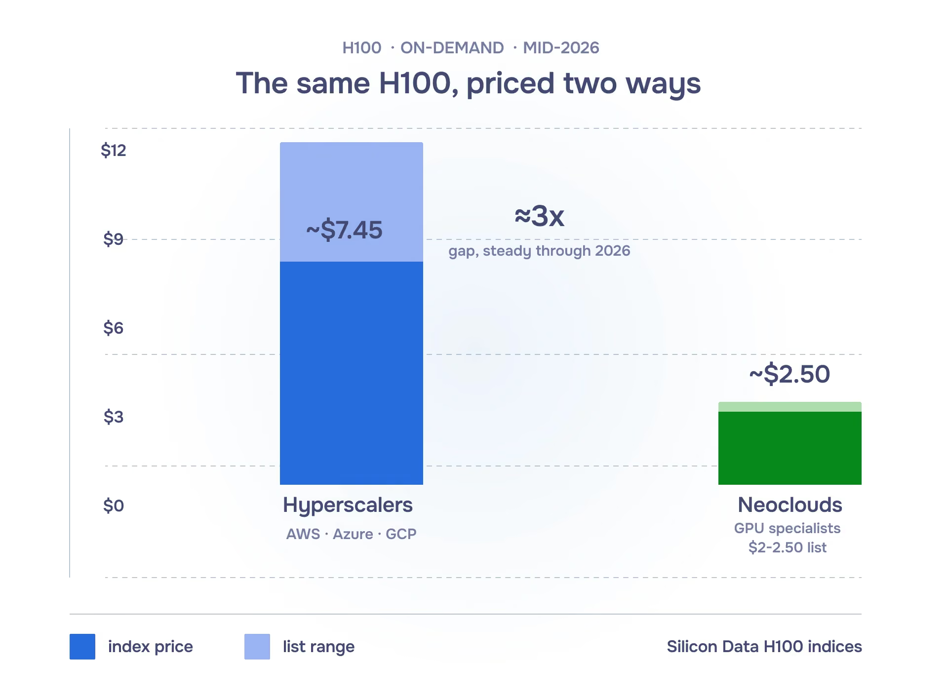
The premium isn't irrational: it buys enterprise SLAs, compliance certifications, and integration with the managed services your stack may already depend on. If your pipeline is welded to S3, BigQuery, or your provider's IAM, the egress and re-engineering cost of moving can exceed the per-hour saving. But if the workload just needs a GPU with a container on it, you're paying a 3× ecosystem tax for an ecosystem you're not using.
The second thing the catalogue doesn't tell you is that price lists assume availability, and 2026 hasn't cooperated. SemiAnalysis's rental index work found on-demand GPU capacity effectively sold out across card types in early 2026, one-year H100 contract pricing up almost 40% between October 2025 and March 2026, and new capacity through late summer already booked. In a market like that, the practical decision rules invert from what the spec sheet suggests:
For interruption-tolerant work, the cheapest real option is neocloud spot — with the caveat from earlier that high-demand cards may simply have none. For latency-bound production, on-demand rates across the specialist providers cluster within about 20% of each other, so the deciding factor is which provider has your card in your region, not who's cheapest on paper. And when comparing across card generations, compare cost per job, not cost per hour: an A100 is cheaper hourly, but an H100's 3–5× transformer throughput often makes it cheaper per training run or per million tokens served.
Two rules of thumb close the loop. If you're on a hosted model API today, self-hosting starts to enter the money when your monthly token bill approaches the monthly cost of a dedicated card plus the engineering time to run it — below that line, the API is the right call and no GPU table applies to you. And if you do run your own card, watch utilization: a common break-even between per-second serverless GPU billing and a dedicated instance sits around 30% utilization. An instance idling at 10% is the most expensive GPU you can buy.
It’s tempting to treat infrastructure as a single decision—which GPU should we use? But the constraints that shape LLM workloads don’t resolve to one answer. Memory determines what fits. Bandwidth determines how fast it runs. Concurrency determines how far a card stretches. Interruption tolerance determines what you can pay.
Those forces don’t converge on a single optimal choice. They fragment the problem.
What emerges instead is a portfolio: different workloads placed on different hardware, under different pricing models, each chosen for its specific constraints. User-facing inference gravitates toward stable, on-demand capacity. Batch and offline jobs move toward spot. Long-context or high-concurrency workloads push into higher-memory cards, while smaller models scale out across cheaper ones. The portfolio itself becomes a system to manage.
If that layer is just a collection of per-provider scripts and tribal knowledge, the operational overhead compounds faster than the savings. What started as a cost optimization turns into fragmentation—different deployment paths, inconsistent visibility, and decisions that are hard to reason about globally.
Whatever sits at that coordination layer—internal tooling, a platform, or a person juggling consoles—it needs to do four things well:
If your current setup can’t do those four things, that gap will cost more than any individual GPU pricing decision. It’s a problem worth solving early, while the portfolio is still small—because once it grows, the coordination layer becomes the bottleneck.
(Full disclosure: that coordination layer is what we build at emma—but the checklist holds regardless of how you implement it.)
Match the card to the model's actual memory footprint and the traffic you expect — not to the workload's reputation. Split every pipeline into its latency-sensitive and interruption-tolerant halves, and price them separately. Track cost per outcome — per thousand tokens generated, per document processed, per training run — rather than per GPU-hour, because hourly rates hide utilization and utilization is where GPU budgets actually leak. And assume from day one that you'll run a portfolio across providers, because you will.
If you would like to learn more, you may also want to read: Where Does the Cloud Money Go?
.avif)
.png)